
By Dmitry Pugachevsky, director of Research at Quantifi, Rohan Douglas, CEO of Quantifi, and Roman Bedau, consultant at Deloitte.
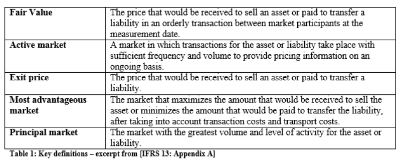
The definitions (see the table 1) are not entity specific and are applied from the perspective of market participants. Therefore, it is necessary for the measurements to take into account all risk factors that influence the fair value.
In this context, the pricing of OTC derivatives still constitutes a complex and challenging task as it has already been under IAS 39.
According to IFRS 13, model-based fair value measurements have to take into account all risk factors that market participants would consider, including credit risk i.e. the counterparty risk for OTC financial products. In order to reflect the credit risk of the counterparty in an OTC-derivative transaction, an adjustment of its valuation has to be made. Therefore, not only does the market value of the counterparty’s credit risk (CVA) need to be taken into account, but also the company’s own counterparty credit risk (debit valuation adjustment - DVA) has to be considered in order to calculate the correct fair value.
Bilateral CVA (The bilateral CVA is calculated by netting CVA and DVA) adjusts the fair value to account for expected losses that result from the default of the counterparty and the company itself (CVA should be evaluated at the netting set level per counterparty). A comprehensive evaluation needs to take into account the time dependent dynamics of the derivatives’ market values as well as an estimate for the probability of default of both contractual partners. Potential correlations between both should be factored into the model too. More common practical approaches waive complex correlation structures and reduce the problem of quantification for the following statistical values:
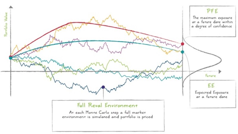
The expected exposure (EE) determines the losses of the surviving contractual party should the counterparty become insolvent. Notably the expected exposure covers collateral agreements defined in the credit support annex (CSA) as well as netting agreements. The best practice methods which determine the expected exposure are Monte-Carlo simulations. Alternatively, less computationally intensive methods based on simpler approximations such as the current exposure with an appropriate add-on term may be applied.
Probabilities of default (PD) and loss given default (LGD) provide an estimation of the probability of a counterparty’s defaults over time. This information can be derived from market noted credit default swap spreads .[1] Additionally, market implicit information can be used to determine the LGD.
Calculating CVA
There is a relatively straightforward approach, occasionally referred to as Quasi CVA, whereby the counterparty credit spread is added to the discount curve applied to the cashflow values of the contract. For example, to evaluate Quasi CVA for 5-year swap, which receives a floating rate of 2% and pays a fixed coupon of 4% for a counterparty with credit spread 3%, one has first to discount cashflows at riskless interest rate (2%), discount them at risk carrying rate (5% = 2% + 3%) and then capture the difference between these two valuations. Note that this method only provides a reasonable approximation of the CVA for instruments with positive cashflows or trades heavily in-the-money. By oversimplifying the calculation, Quasi CVA methodology excludes certain key considerations, for example:
Default losses can be incurred if future MTM is positive, even if current MTM is negative
Market volatility
Bilateral character of CVA (DVA)
Non-linear probability of default and effect of counterparty recovery rate
Wrong way risk
Effects of netting and CSA
The reason that at-the-money or even out-of-the-money swaps produce a non-zero CVA is because CVA is an expectation of future losses, which are incurred by the bank if the counterparty defaults when MTM of the trade is positive. Therefore, CVA is proportional to a zero-strike call option on a future MTM, referred to as Expected Exposure (EE). In general, the exposure of the trade always depends on volatilities of underlying assets, even if the trade itself does not.
When calculating exposures for simple stand-alone instruments like swaps and forwards, one can use European swaptions priced with Black’s formula. However, taking into account netting and collateral requires performing multiple valuations under a host of different scenarios. This allows netted exposure profiles, for any given portfolio of contracts, to be calculated and for collateral to be applied consistently, therefore reducing potential exposure for both counterparties. Specific collateral features to take into consideration include:
Independent amounts
Threshold amounts
Minimum transfer amounts
Call period (frequency at which collateral is monitored)
Cure period (the period of time given to close out and re-hedge a position)
For trades cleared through a central clearing counterparty (CCP), risk specific to that CCP must be considered
Consistent CVA evaluation involves running a Monte Carlo simulation of the market dynamics underlying the valuation of each financial instrument or portfolio. Each market scenario is a realisation of a set of price factors, which affect the value of the financial instrument; for example foreign exchange rates, interest rates, commodity prices, etc. Scenarios are either generated under the real probability measure, where both drifts and volatilities are calibrated to the historical data of the factors, or under the risk-neutral measure, where drifts must be calibrated to ensure there is no arbitrage of traded securities on the price factors. In addition, volatilities should be calibrated to match market-implied volatilities of options on price factors where such information is available.
Having calculated the EE profile, CVA is calculated by multiplying the EE with the probability of default (PD) and loss given default (LGD). CVA can also be approximated by multiplying the average of the EE, the so called Expected Positive Exposure (EPE), by the credit spread and risky annuity. There are several techniques to obtain the credit spread, although the current Basel III requirement is to use CDS credit spreads of the counterparty or its proxy ( N.B. according to IFRS 13.67 those parameters are preferred, which are observable and close to the market.).
Note that the same Monte Carlo simulation can be used for calculating PFE (Potential Future Exposure) and EEPE (Expected Effective Positive Exposure). While PFE is important for calculating Economic Capital and setting internal limits for trading desks, EEPE is part of IMM (Internal Model Method) calculations for deriving RWA (Risk Weighted Asset). Therefore, by building comprehensive Monte Carlo models, consistent valuations for regulatory, accounting and internal limit purposes can be achieved.
The Fair Value adjustment for bilateral credit risk equals risk free valuation, minus CVA plus DVA. Therefore, to complete the calculation one must offset the CVA by the DVA. The DVA is calculated by taking into account the opposite side of the exposure profile (CVA from the counterparty’s perspective). This can be achieved by calculating the Expected Negative Exposure, which can be performed during the same Monte Carlo run without any extra expenditure of time. Common market practice involves taking into account correlation between own and counterparty defaults. This is achieved by either using separate copula-like calculations or as part of a general wrong-way risk set-up. The latter approach makes it easier to incorporate correlations between own default, counterparty default and market factors.
Market Summary
With the introduction of IFRS 13, the requirement to calculate complex variables, such as CVA and DVA remains. . The introduction of IFRS13 will have significant implications for all firms, including corporates and those in the financial services sector that measure financial assets at fair value.